|
IGModel-SW 1.0
|
|
IGModel-SW 1.0
|
This module provides the shallow water equations solver. More...
Functions/Subroutines | |
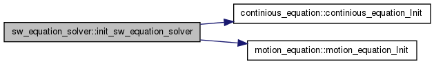
| subroutine, public | init_sw_equation_solver (icgrid) |
| Initialize the sw_equation_solver module. | |
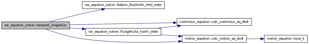
| subroutine, public | temporal_integration (tstep, dt, icgrid) |
| Performs time integration of the shallow water equations. | |
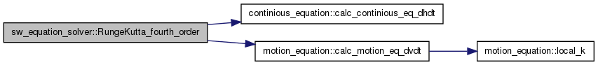
| subroutine | RungeKutta_fourth_order (xy_VelA, xy_VelN, DVelDtN, xy_HeightA, xy_HeightN, DHeightDtN, dt, icgrid, idMin) |
| Performs time integration of the shallow water equations using the forth-order Runge=Kutta method. | |
| subroutine | Adams_Bashforth_third_order (U_nplus1, U_n, dUdt_n, dUdt_nminus1, dUdt_nminus2, dt) |
| Performs time integration of the shallow water equations using the third-order Adams-Bashforth method. | |
This module provides the shallow water equations solver.
Copyright (C) GFD Dennou Club, 2011-2012. All rights reserved.
license ??
| subroutine sw_equation_solver::Adams_Bashforth_third_order | ( | real(DP),dimension(:,:,:,:),intent(inout) | U_nplus1, |
| real(DP),dimension(:,:,:,:),intent(in) | U_n, | ||
| real(DP),dimension(:,:,:,:),intent(in) | dUdt_n, | ||
| real(DP),dimension(:,:,:,:),intent(in) | dUdt_nminus1, | ||
| real(DP),dimension(:,:,:,:),intent(in) | dUdt_nminus2, | ||
| real(DP),intent(in) | dt | ||
| ) | [private] |
Performs time integration of the shallow water equations using the third-order Adams-Bashforth method.
In this subroutine, the future physical fields at  (time level n+1) will be predicted in terms of the fields at current time level n and the local time derivatives of fields at current and previous time levels(n, n-1, n-2).
The value of fields at time level n+1 at all grid-points will be predicted using the equation as
![\[ \Dvect{U}_{n+1} = \Dvect{U}_n + \dfrac{1}{12} \Delta t \left[ 23 \left(\DP{\Dvect{U}}{t}\right)_{n} - 16 \left(\DP{\Dvect{U}}{t}\right)_{n-1} + 5 \left(\DP{\Dvect{U}}{t}\right)_{n-2} \right] \]](form_19.png)
| [in,out] | U_nplus1 | The array in which the physical field data at time level n+1 is stored. |
| [in] | dUdt_n | The array in which the local time derivative data of the physical field at time level n is stored. |
| [in] | dUdt_nminus1 | The array in which the local time derivative data of the physical field at time level n-1 is stored. |
| [in] | dUdt_nminus2 | The array in which the local time derivative data of the physical field at time level n-2 is stored. |
| [in] | dt | Time step [s]. |
Definition at line 469 of file sw_equation_solver.f90.

| subroutine,public sw_equation_solver::init_sw_equation_solver | ( | type(IcGrid2D_FVM),intent(inout) | icgrid | ) |
Initialize the sw_equation_solver module.
| [in,out] | icgrid | The variable of derived type IcGrid2D_FVM. |
Definition at line 103 of file sw_equation_solver.f90.

| subroutine sw_equation_solver::RungeKutta_fourth_order | ( | real(DP),dimension(:,idmin:,idmin:,:),intent(inout) | xy_VelA, |
| real(DP),dimension(:,idmin:,idmin:,:),intent(in) | xy_VelN, | ||
| real(DP),dimension(:,idmin:,idmin:,:),intent(inout) | DVelDtN, | ||
| real(DP),dimension(:,idmin:,idmin:,:),intent(inout) | xy_HeightA, | ||
| real(DP),dimension(:,idmin:,idmin:,:),intent(in) | xy_HeightN, | ||
| real(DP),dimension(:,idmin:,idmin:,:),intent(inout) | DHeightDtN, | ||
| real(DP),intent(in) | dt, | ||
| type(IcGrid2D_FVM),intent(in) | icgrid, | ||
| integer,intent(in) | idMin | ||
| ) | [private] |
Performs time integration of the shallow water equations using the forth-order Runge=Kutta method.
In this subroutine, the future physical fields at (time level n+1) will be predicted in terms of the fields at current time level n.
The future physical field will be predicted using the following equation as
![\[ \Dvect{V}_{n+1} = \Dvect{V}_n + \dfrac{\Dvect{k}_1 + 2\Dvect{k}_2 + 2\Dvect{k}_3 + \Dvect{k}_4}{6} \]](form_13.png)
Where  is a set of variables of velocity and surface height field.
  are functions which represent righ-hand sides of semi-discrete equation of motion, and continious equation, respectively. Then, a set of the functions is defined as
  .
.  are defined as

| [in,out] | xy_VelA | The array in which the velocity field data at time level n+1 is stored. |
| [in] | xy_VelN | The array in which the velocity field data at time level n is stored. |
| [in,out] | DVelDtN | The array in which the time rate of change of velocity field data at time level n is stored. |
| [in,out] | h_nplus1 | The array in which the surface height field data at time level n+1 is stored. |
| [in] | h_n | The array in which the surface height field data at time level n is stored. |
| [in,out] | dhdt_n | The array in which the time rate of change of surface height field data at time level n is stored. |
| [in] | dt | Time step [s]. |
| [in] | icgrid | The variable of derived type IcGrid2D_FVM. |
| [in] | idMin | The lower bound index of arrays in which various physical fields data is stored. |
Definition at line 299 of file sw_equation_solver.f90.

| subroutine,public sw_equation_solver::temporal_integration | ( | integer,intent(in) | tstep, |
| real(DP),intent(in) | dt, | ||
| type(IcGrid2D_FVM),intent(in) | icgrid | ||
| ) |
Performs time integration of the shallow water equations.
| [in] | tstep | The number of time step. |
| [in] | dt | Time step. |
| [in] | icgrid | The variable of derived type IcGrid2D_FVM. |
Definition at line 137 of file sw_equation_solver.f90.

 1.7.3
1.7.3 
